
fNIRS analysis toolbox series – FieldTrip
Introduction
Here we present FieldTrip, which is a MATLAB analysis toolbox that was originally designed for electrophysiological data analysis. However, FieldTrip supports fNIRS data analysis as well. It contains high-level functions that can be combined in a MATLAB script. It aims at researchers with a background in neuroscience, engineering, optics and physics. Here, we show a simple example of how to go from raw data to a visualization of the average response over trials.
This blog post is part 4 of the Artinis blog post series fNIRS analysis toolbox series.
About FieldTrip
FieldTrip has been mainly developed at the Donders Institute for Brain, Cognition and Behaviour at the Radboud University in Nijmegen, the Netherlands. The development is led by Drs. Robert Oostenveld and Jan-Mathijs Schoffelen, and has received contributions from many external institutes all over the world (e.g., USA, UK, and Sweden). The FieldTrip toolbox is based on MATLAB. This toolbox provides preprocessing and post-processing methods for magnetoencephalography (MEG), electroencephalography (EEG), intracranial electroencephalography (iEEG), and fNIRS analysis, including preprocessing, averaging, time-frequency analysis, anatomical coregistration, source reconstruction of EEG and MEG data, and statistical testing.
The FieldTrip toolbox does not provide a graphical user interface; however, it can be combined with MATLAB scripts in an analysis pipeline. This makes it a good choice for users who are familiar with the MATLAB structure and seek to conduct single- or multi-channel fNIRS signal preprocessing and/or post-processing.
The main capability of FieldTrip for fNIRS data is within- and across-subject analysis in the time domain. This includes signal quality assessment, motion artifact detection, artifact reduction, conversion of changes in optical densities to concentration changes in oxygenated hemoglobin (O2Hb) and deoxygenated hemoglobin (HHb), functional response extraction, epoching data, and time-lock analysis. In addition, this toolbox can provide basic visualizations of the data such as plotting single traces or topographic mapping.
The toolbox can be cited as R. Oostenveld, P. Fries, E. Maris, and J. M. Schoffelen, “FieldTrip: Open source software for advanced analysis of MEG, EEG, and invasive electrophysiological data,” Comput. Intell. Neurosci. 2011, 1–9 (2011).
Installing FieldTrip
Prerequisites
FieldTrip is used within MATLAB and hence it is necessary to have MATLAB installed on your computer.
How to install
Specific instructions on how to install FieldTrip on your computer are available here.
Processing pipeline
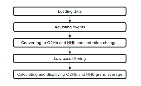
The processing pipeline considered in this tutorial comprises five steps. In the first step, the Artinis fNIRS sample dataset is loaded; details about the dataset can be found in the introduction blog post. In the second step after loading the dataset, we use the event data stored in the dataset to define the events and focus our analyses on the trials where the events took place. In the next step, the optical density signals are converted to O2Hb and HHb signals by using the modified Beer-Lambert law. In the fourth step, the converted signals are cleaned by using a low-pass filter to capture the dynamics in brain hemodynamic response. Finally, the average over trials and the grand average over sessions are computed and the event-related O2Hb and HHb signals are then displayed.
Loading data
To load the data files, we specify the directory and the name of the data files, e.g., in this case:
datafile1 = "c:\Documents\Finger Tapping Experiment\Brite Fingertapping 5-12-2020.oxy4";
datafile2 = "c:\Documents\Finger Tapping Experiment\Brite Fingertapping 5-15-2020.oxy4";
datafile3 = "c:\Documents\Finger Tapping Experiment\Brite Fingertapping 5-19-2020.oxy4";
The text in the quotes should correspond to the full file name (including full path and file extension) of the data recording you would like to load.
To let MATLAB know that we want to use the FieldTrip toolbox and take advantage of the functions embedded, the FieldTrip folder should be added to your path (without subfolders).
In FieldTrip, the dataset is loaded using the ft_preprocessing function. Before calling this function, we need to initialize a configuration variable named cfg. We specify two fields in the configuration variable: the data file location with the file name (datafile1, datafile2, or datafile3) in cfg.dataset; the channel type (‘nirs’) in cfg.channel. The data file is then loaded by calling the ft_preprocessing function with the specified cfg as its argument.
cfg.dataset = datafile1;   % datafile1, datafile2, or datafile3
cfg.channel = 'nirs';
[data_continuous] = ft_preprocessing(cfg);
The data structure that we now have in memory (data_continuous) contains different fields, e.g., channel labels in label; raw fNIRS signals (optical densities) corresponding to the channel labels in trial; time (in seconds) corresponding to the signals in time; the sampling rate of the signals in fsample; information about optodes’ position and type, wavelengths of the transmitters, and the DPF (Differential Pathlength Factor) considered for each channel in opto. See here for more information about the optode information in FieldTrip.close;
Adjusting events
The recorded data used in this blogpost contains three types of events: Rest period, Instructions, and Fingertapping. We aim to analyze the fNIRS data (trials) related to the Fingertapping events. The events are first loaded and adjusted to the fNIRS data which is then segmented into Fingertapping trials. We want to have a look at trials starting 5 seconds before the desired events (pre-stimulus) and ending 30 seconds after them (post-stimulus). We first need to specify some fields of the configuration variable (cfg) left from the previous step (Loading data): the type of event in eventtype and eventvalue, pre- and post-stimulus durations in seconds in trialdef.prestim and trialdef.poststim, respectively. We then call the ft_definetrial function with the adjusted cfg as its argument. The output of ft_definetrial is an updated configuration variable, cfg, in which the events have been loaded and the desired ones (related to the event Fingertapping) have been defined.
cfg.trialdef.eventtype = 'event';
cfg.trialdef.eventvalue = 'Fingertapping';
cfg.trialdef.prestim = 5;
cfg.trialdef.poststim = 30;
cfg = ft_definetrial(cfg);
Next, the data is segmented into Fingertapping trials by calling the ft_redefinetrial function with two arguments: the updated configuration variable, cfg; the data structure with the continuous data, data_continuous. The output of this function is data_epoch in which the field trial contains the segments of the data corresponding to the specified event (Fingertapping).
data_epoch = ft_redefinetrial(cfg, data_continuous);
Converting to O2Hb and HHb concentrations
In this step, we convert the segmented raw data into O2Hb and HHb concentration changes. We first need to initialize the configuration variable and then specify the configuration field target to state the target of the conversion, e.g., one of the options: ‘O2Hb’, ‘HHb’, ‘tHb’ (total hemoglobin), or {'O2Hb','HHb'} (for O2Hb and HHb together). Here we set it to {'O2Hb','HHb'} to obtain both O2Hb and HHb data. Next, we call the ft_nirs_transform_ODs function with the configuration variable, and the segmented raw data. The output of this function is data_conc in which the field trial contains the segmented O2Hb and HHb data with the specified event (Fingertapping).
cfg = [];
cfg.target = {'O2Hb', 'HHb'};
data_conc = ft_nirs_transform_ODs(cfg, data_epoch);
Low-pass filtering
In this step, we apply a low-pass filter with a cutoff frequency 0.1 Hz to remove systemic effects in the data. In the configuration variable, we fill in the field lpfilter with ‘yes’ to enable the low-pass filtering. The cutoff frequency is specified in the field lpfreq in Hz. Finally, we call the ft_preprocessing function with the configuration variable and the data. The output of this function is stored in nirs_Hb_filtered, which contains the filtered O2Hb and HHb data in the trial field.
cfg = [];
cfg.lpfilter = 'yes';
cfg.lpfreq = 0.1;
nirs_Hb_filtered = ft_preprocessing(cfg, nirs_Hb);
Calculating and displaying O2Hb and HHb grand average
In this step, we first want to show how we can compute the average of trials in one session across one specific channel. Then, we show how we can compute the grand average of different sessions across that specified channel.
To compute the average of trials across one specific channel, we specify the channel (‘Rx7-Tx10’) in the field channel of this structure. We add ‘*’ at the end of channel name to consider the different transformations of that specified channel: O2Hb (channel label Rx7-Tx10 [O2Hb]) and HHb (channel label Rx7-Tx10 [HHb]). Hereby two average signals will be computed: one for O2Hb and the other for HHb. To compute the average signals, we call the ft_timelockanalysis function with the configuration variable and the filtered O2Hb and HHb data. The output of this function is stored in the variable timelock in which the fields avg and label contain the average signals and their corresponding labels.
cfg = [];
cfg.channel = 'Rx7-Tx10*';
timelock = ft_timelockanalysis(cfg, nirs_Hb_filtered);
Prior to computing the grand average of different sessions, we will correct the baseline for the average signals obtained. We take the first five seconds of the average signals as the baseline by setting the field baseline to [-5 0]. We then call the ft_timelockbaseline function with the configuration variable and the output of the ft_timelockanalysis function. The output of the ft_timelockbaseline function is stored in the variable timelockbc1, in which the fields avg and label contain the average signals after baseline correction and their corresponding labels.
cfg = [];
cfg.baseline = [-5 0];
timelockbc1 = ft_timelockbaseline(cfg, timelock);
Next, we will compute the grand average of different sessions. For this we need to conduct the same analysis as above for the other two datasets by following the previous steps and store the output of the last step in the respective variables timelockbc1, timelockb2 and timelockbc3.
Finally, having computed the average across the trials in each of the three recordings, we can compute the grand average over the three recordings by calling the ft_timelockgrandaverage function with four arguments: an empty configuration variable and the average data for the three data files: timelockbc1, timelockbc2, and timelockbc3. The output of the grandavg function is the grand average of the three data files across the specified event (Fingertapping) and channel (Rx7-Tx10), It includes the fields avg and label that contain the average signals and their corresponding labels.
cfg = [];
grandavg = ft_timelockgrandaverage(cfg, timelockbc1, timelockbc2, timelockbc3);
Below we plot the O2Hb and HHb grand average signals of channel Rx7-Tx10 from 5 seconds before to 30 seconds after Fingerapping event onset in red and blue, respectively.
channel_name = 'Rx7-Tx10';
O2Hb = grandavg.avg(1,:);
HHb = grandavg.avg(2,:);
figure;
plot(grandavg.time, O2Hb, 'r');
hold on;
plot(grandavg.time, HHb, 'b');
hold off;
title(sprintf('Grand average across channel %s', channel_name));
legend('O2Hb', 'HHb');
ylabel('\DeltaHb (\muM)');
xlabel('Time (s)');

Conclusion
In this blog post, we demonstrated how to use the FieldTrip toolbox for a basic fNIRS analysis. We presented the general toolbox structure and presented an analysis script in MATLAB that results in the event related average for a single channel of one specific event. Hopefully, this blog post provided you with some insights about the possibilities and strengths of the toolbox and helped you to decide if it is suitable for the fNIRS analysis of your interest.
Suggested further reading
There are currently two fNIRS specific tutorials on the FieldTrip website. These tutorials give a general introduction into the basic fundamentals of FieldTrip for fNIRS signal analysis in both single- and multi-channel fNIRS signals.
See also https://www.fieldtriptoolbox.org/getting_started/artinis/
In this blog post, we present MNE-NIRS, a Python toolbox for analyzing NIRS/fNIRS data, which aims at researchers with a background in engineering, neuroscience and/or AI. The toolbox is handled by scripting the processing pipeline, which can be done in a regular Python script or within a Jupyter notebook.