
fNIRS analysis toolbox series – Homer
– Renata Di Lorenzo, Stephen Scott Tucker, & Jörn M. Horschig –
Introduction
Here we present Homer3, an open-source MATLAB toolbox for analysis of fNIRS data and for creating maps of brain activation. Note that you can run the Homer3 executable if you do not have MATLAB (find here for instructions). The toolbox is handled by a graphical user interface (GUI) but also allows the user to export and visualize processing scripts in Matlab. Homer3 aims at researchers with a background in engineering, neuroscience, psychology, and physics.
Here, we present the basic principle of Homer3 and show a simple example of how to read data, preprocess the data (filtering only), average over trials as well as over subjects, and plot the final result in a graph. Suggestions for further reading and tutorials can be found below.
This blog post is part 5 of the Artinis blog post series fNIRS analysis toolbox series.
About Homer3
Homer3 is a continuation of the work on the well-known software Homer2. Specifically, Homer3 arises from the development of the Photon Migration Imaging toolbox in the early ‘90s, which then became Homer, followed by Homer2. The main developers of Homer are David Boas, Jay Dubb, and Ted Huppert, while several other people also contributed to writing specific function codes.
Homer3 comes with a very intuitive and clear main GUI, which allows new Homer3 users to quickly find out how to process fNIRS data. The main features of Homer3 include the ability to write and run .snirf files (read here more about snirf format); three levels of analyses, that is run (i.e. session), subject and group-level analyses; processing functions most commonly used to build up streams for each analysis level; plot of run/subject/group results; export of subject and group hemodynamic response functions (HRF).
Several scientific papers used and tested processing pipelines using the previous versions of Homer; some of these are reported at the end of this blog. The pipelines proposed in these references can be taken as a starting point to build new processing streams in Homer3. The Homer community is quite wide, and as it was for Homer2, also for this newer version, the software issues can be discussed on the Homer3 community forum on openfnirs.org. Issues can be posted on Git Hub by the users; this way, developers and users contribute to improving the software together.
It is worth mentioning that Homer3 is compatible with AtlasViewer, which is a MATLAB toolbox that allows the display of the fNIRS data processed via Homer on anatomical atlases. This toolbox is developed by the Boston University Neurophotonics Center. Here you can find a tutorial on how to perform image reconstruction using AtlasViewer.
How to cite Homer: Huppert, T., Diamond, S., Franceschini, M., Boas, D. (2009). HomER: a review of time-series analysis methods for near-infrared spectroscopy of the brain. Applied optics 48(10).https://dx.doi.org/10.1364/ao.48.00d280
Installing Homer3
Prerequisites
Homer3 can be used within Matlab or as executable, in this last case Matlab is not needed.
How to install
Specific instructions on how to install Homer3 on your computer are reported here
Using Homer3
Figure 1 shows the simplified processing stream that we used in this blog to show some of Homer3 features.
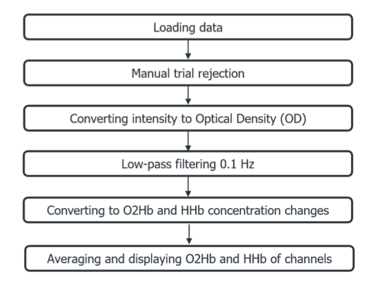
Figure 1. Flowchart example of the processing stream used in this blogpost.
Implementing the processing pipeline in Homer3
Figure 2 displays an overview of the different elements of the main user interface of Homer3. This main window is the persistent part of the GUI, while additional GUIs are opened through the main window to handle specific tasks such as editing events and visualizing subject or group averages.

Figure 2. Overview of the main GUI of Homer3. Labels In dark green describe the different parts of the GUI.
Loading data in Homer3
To load data into Homer3, you need to have .nirs or .snirf files available in a folder which is added to the matlab current directory. To convert .oxy into .nirs files check out this video tutorial.
Individual .snirf or .nirs files are called Runs in Homer3. Runs are optionally organized into Subjects via subfolders, which are in turn organized in Groups. Processing can be carried out across the Run, Subject, or Group level, depending on the selection made in the lower left of the GUI.
Once Homer3 is also added to the Matlab path, all that is needed is to type Homer3 in the Command Window. Next, Homer3 will search for .snirf files, if there are only .nirs files in the selected folder, all .nirs files will be converted to .snirf and loaded in Homer.
After that, Homer3 will look for a configuration file, i.e. .cfg. This file stores the processing stream, if you haven’t created one yet, Homer 3 will load the default .cfg.
All appropriate files in the current MATLAB working directory are reported in the main GUI (see Figure 2, bottom-left corner).
Manual rejection of trials
There are few ways to reject manually invalid or noisy trials from the analysis. One way consists in, first, ticking the box “Edit Excluded Time” in the “Exclude Data” section of the Main GUI, and next drawing a pink window around the events within the Data window. The excluded trials/events will now be displayed as dotted lines (see second pink window in Figure 3). You can also adopt this strategy to exclude manually the time where an artifact occurred (see first pink window in Figure 3). To better visualize data and artifacts the user can zoom in the ‘Data Window’.
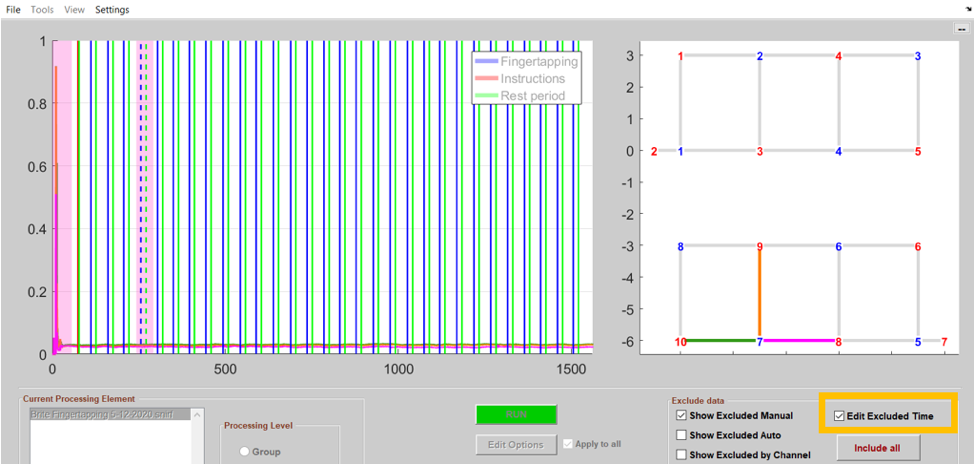
Figure 3. Example of manually excluded time series via the Edit Excluded Time button. The first pink window shows excluded time due to artifacts, while the second displays trial-rejection.
Channel rejection can be also performed manually by left clicking on the channel in the Probe Window. Also, in this case, the excluded channel will be displayed as dotted line (See Figure 4)

Figure 4. Example of a manually excluded channel.
Creating a processing stream
To process the data, a processing stream must be created. This can be done via Tools > Edit Processing Stream. Another GUI will pop-up showing all functions available to process data at a run, subject, and group level. A detailed explanation of the selected function is also provided (see Figure 5).
In this GUI the user can create and modify the processing stream. Once the processing stream is created, the user can load it to the current dataset by clicking Save > Current Processing Stream, or save it to disk as .cfg via Save > Config file. This .cfg file can be shared with colleagues, to share a common processing pipeline in Homer3. A .cfg file can be loaded to the current dataset using the Load button in this GUI (Load > Config file).

Figure 5. Processing Stream GUI showing the Run/session processing options.
Once the processing stream is loaded to the current dataset, the user can adapt the parameters of each function from the main GUI (see Figure 2, Edit Option in the preprocessing field).
Converting Intensity to ODs
First step in the processing stream is the conversion to ODs. This step does not require the definition of any parameter.
Low-pass filtering 0.1Hz
Several functions in Homer run on OD data, such as the band-pass filter. To enable only the low-pass filter at 0.1 Hz, the hpf needs to be set to 0 and lpf to 0.1. This filter is a third order Butterworth.
MBLL - Conversion from ODs to hemoglobin concentration changes
In this step the Modified Beer-Lambert Law is applied. The conversion from ODs to Concentration changes requires the user to insert ppf values corresponding to each wavelength (partial pathlength factor, also called DPF, differential path length factor). These are age and wavelength specific. Here we use 6.06.
Averaging of trials
Averaging of trials is done on Concentration data and requires the definition of a time window. Here we use -5 (i.e. 5s prior to stimulus onset) to 30s (i.e. after stimulus onset). The 5s prior to stimulus onset are used for later baseline correction.
Plotting trial average
There are two ways to visualize the trial averaged data. If you want to see the averages at a channel base, tick the HRF box, select the condition, and the channel of interest in the Probe Window. Select the View HRF Std Error option in the View menu to visualize the standard error relative to the trials (e.g. see channel Rx7-Tx10 displayed in Figure 6).

Figure 6. The left panel shows oxy- and deoxy hemoglobin averages (HbO and HbR in Homer) and relative error bars of one channel of one session/subject. The right panel indicates in green channel Rx7-Tx10, which data is shown in the left panel.
To visualize all channels of one recording simultaneously, select from the main toolbar Tools > Plot Probe. A PlotProbeGUI will pop-up displaying all channels’ HRF (see Figure 7).

Figure 7. Subject/Session Averages of Oxy (in red), Deoxy- (in blue), and Total-hemoglobin (in green; HbT in Homer) of all channels.
To average all trials across sessions or within a group, you first need to process the session/group data. To do that, on the main GUI menu bar, click on Tools>Edit Processing Stream. The ProcStreamEditGUI pops-up, here click on the Group tab and select the preferred options, then save to the current processing stream and close the GUI (Figure 8).

Figure 8. Processing Stream GUI showing the Group processing options.
In the main GUI select Group as Processing level and click on Edit options to visualize the processing stream for Group analyses. Next, click on Run. Once the processing is done, you can visualize in the main GUI (see Figure 9) or in the PlotProbeGUI the Group/Session Results (see Figure 10).
By clicking on the menu bar File>Export you can easily export data from Homer in .txt to perform statistics in your preferred program (see Figure 9). It is possible to export the HRF data or the Subject HRF mean.

Figure 9. Group average and Std Err bars of oxy- (bold line) and deoxy-hemoglobin (thin line) traces. The window on the right shows up when clicking on File>Export> Subject HRF mean, here it is possible to select the time range. It is also possible to export the HRF data for the current data file selected or all files, as well as the processing stream script as .m file.

Figure 10. Group Averages of Oxy (in red), Deoxy- (in blue), and Total-hemoglobin (in green) of all channels.
Conclusion
This was a brief overview of a basic processing pipeline in Homer3.
Homer3 allows users to easily create a processing stream for session, subject, and group. The processing GUI explains how each function works so the user can better grasp how to properly apply it to the data. Further, original data are never modified but after processing the results are stored for each processing step, the original data are retained and the results are automatically given descriptive names. This makes it very easy to keep track of what has been done and backtrack if needed.
Due to Homer3's intuitive GUI design and the fact that users do not need to manually code to process data, Homer3 proves a great pre-processing tool for fNIRS data, especially for users new to the technique. Yet, more expert users can also export the processing stream as a Matlab file and tailor their processing steps.
One of the strengths of Homer is the online support behind it. That is, users and developers exchange opinions, feedback, and issues here which also helps improve the next software versions.
Suggested further reading
To get some inspiration on fNIRS processing pipelines check out these studies that used Homer to evaluate their effectiveness on different participants samples and tasks.
Pipeline tested on: