
fNIRS analysis toolbox series – MNE/Python
– Sofia Sappia, Liza Genke, Robert Luke, & Jörn M. Horschig –
Introduction
In this blog post, we present MNE-NIRS, a Python toolbox for analyzing NIRS/fNIRS data, which aims at researchers with a background in engineering, neuroscience and/or AI. The toolbox is handled by scripting the processing pipeline, which can be done in a regular Python script or within a Jupyter notebook.
Here, we present the basic principles of MNE and show a simple example of how to read NIRS data, preprocess it and run and plot an average over trials and sessions. Suggestions for further reading and tutorials can be found below. This blog post is also available as a notebook, which you can follow here.
This blog post is the final part of the Artinis blog post series fNIRS analysis toolbox series.
About MNE-NIRS
MNE-NIRS is an open-source toolbox for Python, developed by Robert Luke, Eric Larson and Alexandre Gramfort. It was originally designed for exploring, visualizing, and analyzing human electrophysiology data, but currently supports human brain hemodynamic time series data. MNE offers comprehensive analysis tools and workflows that allow users to assemble complete data analysis pipelines that encompass most phases of NIRS data processing. MNE-NIRS does not run in the form of a GUI but is handled by scripting in the processing pipeline, which provides more flexibility for users comfortable programming in Python.
MNE-NIRS shares common functionalities with MNE-Python toolbox, which is why its documentation is split into MNE-NIRS API reference website, for specific NIRS functions in the toolbox, and in MNE-Python API reference one, for general functions common to either EEG or EMG data analysis functionalities. In addition, several examples are available on the MNE NIRS website, which are useful for getting started with different kinds of analysis. Both MNE-Python and MNE-NIRS are actively maintained and updated, and there is a growing active community using both toolboxes and interacting through the MNE Forum.
To cite the MNE-Python package, please use:
In this blog post, we will take in-house recorded data with a finger-tapping experiment and will guide you through a simple analysis pipeline using MNE-Python and MNE-NIRS. Before getting started with this short guideline, we suggest you check out the installation instructions.
Using MNE-NIRS
The general workflow that we will present today includes a step for loading the data, followed by a visual inspection of it and the rejection of bad trials. We will preprocess the data by applying a low pass filter and will then convert the raw optical densities into concentration changes in oxygenated (O2Hb) and deoxygenated (HHb) haemoglobin. Please note that O2Hb and HHb signals are respectively named as HbO and HbR in the toolbox. We will segment O2Hb and HHb signals into trials to perform an average over trials for each session and, in the final step, we will also perform an average over sessions.

Loading the data
To load the oxy4 NIRS data on MNE-NIRS, simply use convert_oxy4_to_MNE_Raw function, which will load the data into the MNE data object “raw_od”. Bear in mind that Oxysoft should be installed in your PC and registered as a DCOM-interface for this function to run. Once you have your raw_od object, use pick_types mne function to select NIRS data only. This object contains all the NIRS channels recorded in the experiment, as well as information about the onsets and types of events.
fname = "Brite Fingertapping 5-12-2020.oxy4"
raw_od = convert_oxy4_to_MNE_Raw(fname)
Manual rejection of trials
Visual inspection of the data allows us to identify channels or trials where signal quality is not good enough for analysis. For this, we can use the plot function embedded in our MNE data object. In this example, we illustrate the visual inspection of a short segment of 120 s of duration, starting from the Instructions event onset and including 5 fNIRS channels. If using Jupyter notebook, we suggest you use the matplotlib inline widget to interact with the plots. You can use the scrollbars and zoom button to navigate the data and check their signal quality.
%matplotlib inline
%matplotlib widget
tstart = raw_od.annotations.onset[(raw_od.annotations.description) == 'Instructions']
raw_od.plot(n_channels=len(raw_od.ch_names), duration=120, show_scrollbars=True,
scalings='auto', clipping=None, start=tstart);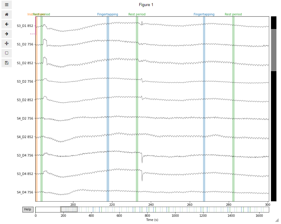
Figure 1. Visualization of raw optical densities in MNE-nirs toolbox as seen using matplotlib inline widget for a set of channels.
Low-pass filtering 0.1Hz
The function “filter” in our MNE data object allows for designing and applying various types of filters. In this example, to implement a low pass filter of 0.1 Hz, we set the low cutoff and high cutoff frequencies at None and 0.1 Hz, respectively. We choose a finite impulse response filter with the following parameters, which will be automatically displayed when running the command:
filt_ODs = raw_od.filter(None, 0.1, h_trans_bandwidth=0.2, l_trans_bandwidth=0.02)FIR filter parameters
Designing a one-pass, zero-phase, non-causal low-pass filter:
Windowed time-domain design (firwin) method
Hamming window with 0.0194 passband ripple and 53 dB stopband attenuation
Upper passband edge: 0.10 Hz
Upper transition bandwidth: 0.20 Hz (-6 dB cutoff frequency: 0.20 Hz)
Filter length: 165 samples (16.500 sec)
To visualize the resulting signals we proceed as follows:
filt_ODs.plot(n_channels=len(filt_ODs.ch_names[:10]),
   duration=120, show_scrollbars=True,
      scalings='auto', clipping=None, start=tstart
         );

Figure 2. Visualization of low-pass filtered NIRS data in MNE-NIRS toolbox.
MBLL - Conversion from ODs to hemoglobin concentration changes
The third step in our preprocessing pipeline is the conversion of the optical density signals into changes in oxygenated (O2Hb) and deoxygenated (HHb) haemoglobin. For this conversion, we can choose to specify the partial pathlength factor (PPF), which is a combination of the differential pathlength factor (DPF) and the partial volume correction (PVC): PPF = DPF/PVC. We choose a PPF value of 6 and apply the Modified Beer-Lambert Law as follows:
raw_haemo = mne.preprocessing.nirs.beer_lambert_law(filt_ODs, ppf=6)The converted O2Hb and HHb signals are stored in our new raw_haemo MNE data object. To visualize these signals, we proceed as explained in the previous step. O2Hb and HHb signals are automatically represented in red and blue traces, respectively.
raw_haemo.plot(n_channels=len(raw_haemo.ch_names[:10]),
   duration=120, show_scrollbars=True,
      scalings='auto', clipping=None, start=tstart);

Figure 3. Visualization of O2Hb(A) and HHb (B) signals in MNE-NIRS.
Averaging of trials
Identifying events from the experiment design
We will perform the average over trials on the hemoglobin concentration changes. To do so, we need to define a time window based on our experiment design. As a first step, we identify the three different events in our data: “Fingertapping”, corresponding to the task; “Instructions”, marking the start of the experiment; “Rest period”, corresponding to the start of each rest period. We save them in a dictionary event_dict, and plot them with the plot_events function of the visualization module of MNE for an overview of the experiment design.
events, event_dict = mne.events_from_annotations(raw_haemo)fig = mne.viz.plot_events(events, event_id=event_dict, sfreq=raw_haemo.info['sfreq'])fig.subplots_adjust(right=0.7) # make room for the legend
Figure 4. Visualization of events in MNE-NIRS.
Segmenting the data into trials
We will consider trials starting from 5 seconds before stimulus onset (tmin = - 5) until 30 seconds (tmax = 30) of trial duration, after stimulus onset. We use the Epochs method in MNE to segment the data into trials (“epochs”). The 5 seconds before the stimuli are used for baseline correction of O2Hb and HHb signals on each trial.
tmin, tmax = -5, 30
epochs = mne.Epochs(raw_haemo, events, event_id=event_dict,
      tmin=tmin, tmax=tmax,
   proj=True, baseline=(tmin, 0), preload=True,
   detrend=None, verbose=True)
The previous data segmentation was applied on all channels in our data. For visualization purposes, we will also compute it on a single channel. We choose “S10_D7” and select it by means of the “pick_channels_regexp” method. However, in order not to overwrite our previous data, we will make a copy raw_haemo and name it “single_haemo”. We will then use this object for single channel analysis.
single_haemo = raw_haemo.copy()
picks = mne.pick_channels_regexp(single_haemo.ch_names, regexp='S10_D7')
raw_haemo.plot(order=picks, n_channels=len(picks), duration=120, show_scrollbars=True,
      scalings='auto', clipping=None, start=tstart);
sep_ch = single_haemo.pick(picks)

Figure 5. Visualization of O2Hb and HHb signals in channel S10_D7 in MNE-NIRS.
We proceed with the segmentation as explained for all channels.
epochs_single = mne.Epochs(sep_ch, events, event_id=event_dict,
   tmin=tmin, tmax=tmax,
   proj=True, baseline=(tmin, 0), preload=True,
   detrend=None, verbose=True)
Plotting average
We are now able to select the trials corresponding to the finger tapping task and plot both HHb and O2Hb average over trials.
For the single channel case:
evoked_dict = {'O2Hb': epochs_single['Fingertapping'].average(picks='hbo'),
               'HHb': epochs_single['Fingertapping'].average(picks='hbr')
              }

# Rename channels until the encoding of frequency in ch_name is fixed
 for condition in evoked_dict:
      evoked_dict[condition].rename_channels(lambda x: x[:-4])

color_dict = dict(O2Hb='#AA3377', HHb='b')

mne.viz.plot_compare_evokeds(evoked_dict, ci=0.95,
      colors=color_dict);

Figure 6. Average over trials for O2Hb and HHb signals in channel S10_D7 in MNE-NIRS.
Similarly, for all channels:
epochs['Fingertapping'].plot_image(combine='mean')

Figure 7. Average over trials for O2Hb (A) and HHb (B) signals from all channels in MNE-NIRS.
Plotting average over sessions
To plot the average over sessions, we run the pipeline for each session dataset. We save in different variables the data segmented into trials. We chose to name the files as “epochs_session1”, “epochs_session2”, and “epochs_session3” for sessions 1, 2 and 3, respectively. Afterwards, we proceed as explained for a single session and save the data for each session in the “sessions_dict” dictionary.
sessions_dict = {'O2Hb': epochs_session1['Fingertapping'].average(picks='hbo'),
   'O2Hb': epochs_session2['Fingertapping'].average(picks='hbo'),
   'O2Hb': epochs_session3['Fingertapping'].average(picks='hbo'),
   'HHb': epochs_session1['Fingertapping'].average(picks='hbr'),
   'HHb': epochs_session2['Fingertapping'].average(picks='hbr'),
   'HHb': epochs_session3['Fingertapping'].average(picks='hbr')
  }

# Rename channels until the encoding of frequency in ch_name is fixed
 for condition in sessions_dict:
   sessions_dict[condition].rename_channels(lambda x: x[:-4])

color_dict = dict(O2Hb='#AA3377', HHb='b')

mne.viz.plot_compare_evokeds(sessions_dict, ci=0.95,
   colors=color_dict, combine='mean');

Figure 8. Average over sessions for O2Hb and HHb signals in channel S10_D7 in MNE-NIRS.
Conclusion
In this blog post, we have learned about the MNE-NIRS toolbox and how it can be used to perform a simple pipeline for NIRS data analysis and visualization. MNE-NIRS offers many modules and functionalities that encompass several data analysis steps for analyzing functional NIRS data. We recommend MNE-NIRS to engineers, psychologists, and neuroscientists comfortable with programming in Python language and who enjoy the flexibility and practicality of a toolbox that is designed to be handled by scripting the processing pipeline. We suggest you combine its capabilities with mathematical Python libraries, such as NumPy and scikit-learn.
Lastly, we provide you with some sample publications from groups already using MNE-NIRS for NIRS data analysis:
In this blog post, we present MNE-NIRS, a Python toolbox for analyzing NIRS/fNIRS data, which aims at researchers with a background in engineering, neuroscience and/or AI. The toolbox is handled by scripting the processing pipeline, which can be done in a regular Python script or within a Jupyter notebook.