
fNIRS analysis toolbox series – Brain AnalyzIR
Introduction
Here we present the NIRS Brain AnalyzIR toolbox, a toolbox for analysis of (f)NIRS data in Matlab. The toolbox is based on an object-oriented programming paradigm and is handled by scripting the processing pipeline in Matlab. NIRS Brain AnalyzIR toolbox aims at researchers with a background in neuroscience. The toolbox is suitable for researchers who have basic knowledge of Matlab and especially those who are comfortable with object-oriented programming.
Here, we present the basic principles of the toolbox and show a simple example of how to read the data and prepare it for analysis by adjusting events and converting raw optical density (OD) values to hemoglobin concentrations. Furthermore, we will demonstrate how to perform two types of analysis: applying a General Linear Model (GLM) and deriving the grand average of hemodynamic response over the total number of event trials in a study. Suggestions for further reading and tutorials can be found below. This blog post is part 3 of the Artinis blog post series fNIRS analysis toolbox series.
About NIRS Brain AnalyzIR Toolbox
The NIRS Brain AnalyzIR toolbox is an academic open-source toolbox for Matlab, developed by the Huppert Brain Imaging Lab (University of Pittsburgh) led by Dr. Theodore Huppert. The main developers of the toolbox are Theodore Huppert, Jeffrey Barker, Frank Fishburn, and Xuetong Zhai. The data processing in the toolbox is accomplished by using a command-line interface to call functions and pass an object representation of the fNIRS data. There is also a growing number of visualization graphical interfaces available for visualizing data and preparing analysis scripts. In the toolbox, the processing modules (functions) are combined to form an overall analysis pipeline. For certain functionalities, e.g., modifying stimuli information and displaying the data, graphical user interfaces (GUIs) are provided. The toolbox was created as a package of statistical analysis particularly tailored for fNIRS data. Specifically, the toolbox provides a rather straightforward implementation of the first and higher level (group) statistical analysis while taking into account the spatially and temporally structured noise to prevent statistical fallacies. Some of the common noise characteristics and statistical assumptions for (f)NIRS analysis are reviewed in Huppert (2016). The commentary emphasizes the importance of using statistical models tailored to these NIRS-specific issues.
The core functionalities are introduced in an introductory NIRS Brain AnalyzIR toolbox paper: Santosa et al., 2018. Although there is no extensive documentation on how to use each function, most of the toolbox functions have explanations in them as comments and sometimes include examples of usage. The toolbox allows one to script the analysis once and apply it to multiple subjects. In addition to a variety of data processing functions, the toolbox folder contains examples of analysis pipeline scripts that are useful for getting started with a new project. Furthermore, there are multiple tutorials online and active communities on social media to assist in gaining experience with the NIRS Brain AnalyzIR toolbox. The toolbox is actively maintained and updated by the authors. Another advantage of the toolbox is the possibility to interact with other functions from Matlab-based (f)NIRS analysis toolboxes: HOMER2, NIRS-SPM, Fieldtrip, and their functions. This allows the toolboxes to complement each other and the user can compare various analysis options.
The toolbox can be cited as Santosa, H., Zhai, X., Fishburn, F., & Huppert, T. (2018). The NIRS brain AnalyzIR toolbox. Algorithms, 11(5), 73.
Installing NIRS Brain AnalyzIR Toolbox
Prerequisites
The toolbox requires Matlab version 2014b or higher. Most of the toolbox functions run with the basic Matlab program and do not require any additional Matlab toolboxes, although it is advisable to have the Matlab Statistics and Signal Processing toolboxes. Some parts of the analysis (specifically, image reconstruction methods) require downloading additional software: NIRFAST (Near-Infrared light transport in tissue and image reconstruction), Matlab/Octave-based mesh generation toolbox (Iso2mesh), MCextreme (Monte Carlo Extreme). MMC (mesh-based Monte Carlo), or the tMCimg software (Monte-Carlo photon transport) packages.
How to install
The toolbox can be downloaded to your local computer in two ways: by using a Git repository management tool (e.g. TortoiseGit) or by downloading the ZIP file from the website. We will consider the latter option in this tutorial.
Use the link https://github.com/huppertt/nirs-toolbox to access the repository of the toolbox, click the green button and select Download ZIP.
Once the file is downloaded, unzip it in a desired folder, e.g. C:\fNIRS.
To be able to access the toolbox functions, the toolbox folder location needs to be added to the Matlab paths. It can be done by executing two lines in the Matlab command window.
3.1. First, specify the main toolbox folder as toolbox_path. It will depend on the location where the toolbox folder is placed, in this case:
toolbox_path = 'C:\fNIRS\nirs-toolbox';3.2. To add the main folder and subfolders to the Matlab path, enter the line below in the Matlab command window. The command will be executed silently and the toolbox folder with subfolders will be added to the Matlab path.
addpath(genpath(toolbox_path));Alternatively, this step can be performed by using the Matlab Pathtool (find Set Paths button under Home commands or type pathtool on the command line) and i) using Add Folder to navigate to and add the root toobox_path (defined above) and ii) use Add with Subfolders to navigate to and add the demo and external folders inside the root directory.
Before starting, we strongly recommend familiarising yourself with the structure of the subfolders and locations of toolbox functions as they will be necessary to specify to navigate to a particular function. For example, to get the function ANOVA.m, we first need to go to +nirs and then +modules folders: C:\fNIRS\nirs-toolbox\+nirs\+modules. The + sign and the name next to it indicate to which classes the function belongs. We will use these classes (or namespaces) when calling the functions by combining them with the dots as follows: nirs.modules.ANOVA. To learn more about object-oriented programming in Matlab, please see MathWorks.
In Matlab, you can auto-complete a command by starting to type the name of the function and hitting the <TAB> key, which will then display all possible completions to the command. For example, to list all the commands in the module’s namespace, you can type nirs.modules. and hit <TAB>. You should see a popup of all the commands that are in the +modules folder. This is also useful if you cannot remember the exact spelling or name of a function. If you do not see anything when you type nirs. and hit <TAB>, the Matlab path is probably not set properly. To solve it, repeat the steps introduced previously in the blog.
Now you are ready to start working with the toolbox!
Link to manual.
https://bitbucket.org/huppertt/nirs-toolbox/wiki.
Eventually, the toolbox documentation will be available on this site: https://fnirsanalysisclub.org/software/.
Using NIRS Brain AnalyzIR Toolbox
Overview of the planned analysis

After loading the data, a few adjustments will be implemented to exclude the irrelevant recording segments, i.e. parts where the experimental task did not take place. We will also change the duration of the events. The correct duration of the task will be essential to model the HRF for GLM analysis. The original .nirs recording contains raw light intensity values which first need to be converted to OD values. To arrive at a physiologically meaningful signal, the optical densities must be transformed into hemoglobin through the modified Beer-Lambert law (MBLL). These will be the steps of the initial preparation of the data.
Afterwards, two different types of analyses will be performed. In the first analysis, GLM analysis will be performed and the result will be visualized by using built-in toolbox functions.
In the second analysis, we will demonstrate how to interface with Homer2 functions by implementing filtering and averaging of the trials.
Finally, we will demonstrate how to preprocess multiple fNIRS sessions and to place them in a hierarchical folder structure suitable for second order statistical analysis.
Loading data
To load data into BrainAnalyzIR, you can use .nirs or .snirf file available in a folder which is added to the Matlab current directory. To convert .oxy into .nirs files check out this video tutorial. Alternatively, .loadOxy3 can be used to load .oxy3 files directly to the toolbox.
To be able to load the data file of interest, we will first specify the location of the data file and the name of the data file, e.g., in this case:
file = 'C:\Documents\Finger Tapping Experiment\2020-05-15_Finger_Tapping_Brite_S01.nirs';The text in the quotes should correspond to the full file name (including full path and file extension) of the data recording you would like to load.
The toolbox provides a set of functions to read in fNIRS data depending on the file format. All possible options can be found in the C:\fNIRS\nirs-toolbox\+nirs\+io folder. In this tutorial we are using .nirs file, thus, we will call:
raw = nirs.io.loadDotNirs(file); After this step, a variable raw will appear in the Matlab workspace window - it contains the data from the recording. You can now familiarize yourself with the variable fields by double-clicking on the variable in the workspace or by plotting data using raw.draw.
raw.draw;Make sure to close the graph before proceeding to further analysis by manual clicking on the close button or using command close.
close;You can also interactively view the data with the call:
raw.gui;This function will show the data time course and provide a graphical representation of the probe that you can click to select and view different channels.
Adjusting events
We will first discard irrelevant data segments and adjust stimuli durations. To eliminate the data that does not contain information about the experiment, the .TrimBaseline function from nirs.modules can be used by specifying the preBaseline period as 5s before the first event and the postBaseline as 20s after the last event of the experiment:
jobs = nirs.modules.TrimBaseline();jobs.preBaseline = 5; % time before the first event jobs.postBaseline = 20; % time after the last event
To execute a defined job, we will call jobs.run and include the variable to apply the function on in the parentheses (raw). The output of the job in the line below is specified to be raw_exp.
raw_exp = jobs.run(raw);In the variable field raw_exp.stimulus information about the stimulation protocol can be found, e.g., the name, the onset and the duration of the experimental events. To inspect this information we will call a stimulus GUI.
raw_exp = nirs.viz.StimUtil(raw_exp);The following GUI will appear on the screen:

The duration of finger tapping event fields needs to be adjusted, since trials lasted for 15 s during the experiment. It can be done by entering number 15 in each duration field and pressing OK.

Tip💡
Right-click on one of the duration fields, select Set Duration All and enter 15. In case you would like to delete all events with the same name, right click on the name of the respective event in the upper-right list and select Delete Stim.
Converting to O2Hb and HHb concentrations
The NIRS Brain AnalyzIR toolbox provides a convenient way to define the analysis pipeline by creating a list of jobs. In this section we will illustrate how to script the pipeline to convert raw data to O2Hb and HHb concentrations. The analysis pipeline can also be defined by calling nirs.viz.jobmanager command which will open a GUI.
Each job can have an input, specified in parentheses. When initialising the first job in the list, the parentheses should stay empty. For subsequent jobs, the name of the preceding jobs should be added in the parentheses. In this case, it is defined as the variable jobs. This means that all jobs in the list will be executed subsequently by passing the outcome of one job to another.
jobs = nirs.modules.OpticalDensity();jobs = nirs.modules.BeerLambertLaw(jobs);Hb = jobs.run(raw_exp);The .BeerLambertLaw module utilizes the partial pathlength factor (see Strangman et al., 2003) when converting optical densities to concentration changes. After executing the list of jobs, a new variable Hb containing the O2Hb and Hb information will be created in the Matlab workspace. To inspect the data, you can use the nirs.viz.nirsviewercommand.
nirs.viz.nirsviewer
The command will open a Matlab user interface. On the top right of the window you can select and deselect the channels that are drawn. In the panel below it is possible to change the type of a trace (O2Hb and HHb) by clicking on it. The lowest panel indicates which subject’s data is drawn. Feel free to explore other Menu options available in nirs.viz.nirsviewer.
GLM analysis
Now, as we have our stimuli in order, we can continue by applying a GLM analysis on the data. In GLM analysis, a reference function, which consists of a linear combination of regressors, is fitted to the time course of each channel. The design matrix for the GLM reference function is created by convolving the boxcar function (boxcar time course acquires values of 1 when the condition is on and 0 when the condition is off) with the hemodynamic response function. In addition, various other regressors can be added to the model.
In NIRS Brain AnalyzIR toolbox, the GLM analysis can be applied with the following commands:
jobs = nirs.modules.GLM();Hb_GLM = jobs.run(Hb);
Note that the first line initializes a new pipeline rather than extends the one we created previously since it would not make sense to call OpticalDensity and the Beer-Lambert module again on the newly created Hb variable.
Displaying GLM results
To plot the final result we will call .draw function:
Hb_GLM.draw
The color scale in the graphs indicates the t-test value derived based on the beta values of the GLM model. The color of each channel represents a corresponding t-test value. To determine which of the channels have a significant activation, a threshold of the q-values can be specified in the parentheses as follows:
Hb_GLM.draw('tstat', [], 'q<0.05')The first argument in this draw command can be either tstat or beta depending on whether you prefer to draw the statistical effect or the absolute magnitude of the estimate. The second argument (here as <[]>) sets the color scale and is used in case you would like multiple figures to have the same color scale limits. Use the empty set <[]> for autoscaling. Finally, the last argument defines the statistical threshold. You can use p<## or q<## where the letters indicate whether p-values or the Benjamini-Hochberg FDR corrected q-value levels are used and the hashtags should be replaced by the desired threshold.

The solid lines represent the channels for which the q-value is lower than the threshold specified when calling the function.
You can also interact with the data by typing:
Hb_GLM.gui;The GUI will allow you to select which contrast to display and the thresholds.
Low-pass filtering 0.1 Hz
As mentioned in the introduction, NIRS Brain AnalyzIR toolbox allows interfacing with other toolboxes. The following section will demonstrate how to utilize some functions from the Homer2 toolbox for deriving the grand average of O2Hb and HHb for each channel.
To be able to call Homer2 functions from the NIRS Brain AnalyzIR toolbox, it is necessary to have the Homer2 source code on your computer and add it to the Matlab paths. Instructions on how to download the Homer2 scripts and set paths can be found on Homer2 website. Thus, it will not be covered extensively here.
In short, after downloading the source code package, navigate to the Homer2 toolbox directory using the cdcommand, execute the function to setpaths and return back to the NIRS Brain AnalyzIR toolbox directory. In the piece of code below, the directory names should be adjusted in a way that it matches the paths on your computer.
cd 'C:\fNIRS\homer2'setpaths;cd('C:\fNIRS\nirs-toolbox') % navigate back to toolbox folderWe will apply a low-pass filter with a cut-off 0.1 Hz to reduce the noise in the data. If you are familiar with Homer2 Process Stim GUI, you might recall a function hmrBandpassFilt which can be used for this purpose. Homer2 uses a third-order Butterworth IIR filter. In NIRS Brain AnalyzIR toolbox, the same function can be called without the user interface by specifying a cut-off value of the filter as jobs.vars.lpf. Other parameters (e.g. type) of the filter will be set to default values used in Homer2.
jobs = nirs.modules.KeepStims(); jobs.listOfStims = {'Fingertapping'}; % keep finger tapping trials onlyjobs = nirs.modules.Run_HOMER2(jobs);jobs.fcn = 'hmrBandpassFilt'; % indicate the function for applying the bandpass filterjobs.vars.lpf = 0.1; % define the low-pass cut-off frequencyjobs.vars.hpf = 0; % define the high-pass cut-off frequency (0 for no high-pass filter)Hb_filtered = jobs.run(Hb);Note that there is an alternative way to apply a band-pass filter in fNIRS toolbox by usingeeg.modules.BandPassFilter. Feel free to explore this option.
Calculating and displaying O2Hb and HHb grand average
Subsequently, an average of the task trials can be calculated for each channel using the function hmrBlockAvg. The input for this function requires specifying trange. The range defines how many seconds before the task onset (-5) and after the task onset (+30) of the event should be used to calculate the averages.
jobs = nirs.modules.Run_HOMER2(jobs);jobs.fcn = 'hmrBlockAvg';jobs.vars.trange = [-5 30]; % define the time range for averaging with respect to the task onset Hb_avg = jobs.run(Hb);To display the result enter:
Hb_avg.gui;

The upper image shows the O2Hb average and the lower image illustrates HHb average of the finger tapping task trials for different channels.
The visualization of the O2Hb and HHb values in the same graph can be implemented by using .draw() and specifying the channel indices in the parentheses. We chose to plot the Rx7-Tx10 channel as it yielded the highest O2Hb and lowest HHb t-test values in the GLM analysis. First, the O2Hb and HHb channel indices are found using Matlab function find. Afterwards, both of these traces are plotted in a separate figure:
% find channel Rx7-Tx10 indicesch_ind = find(Hb_avg.probe.link.detector == 7 & Hb_avg.probe.link.source == 10); % display grand averageHb_avg.draw(ch_ind)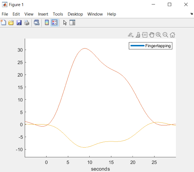
Analyzing multiple sessions
The NIRS Brain AnalyzIR toolbox provides functions to perform, e.g., higher order mixed effects or ANOVA analysis on multiple subjects’ and/or multiple sessions’ data. For this purpose, the folders containing recordings should have a hierarchical structure. We will illustrate how to create a hierarchical structure using multiple sessions acquired from the same subject. First, we will select the root directory and specify it in Matlab as root_dir, for example:
root_dir = 'C:\Documents\Experiment';In this folder, we will create a new folder and name itGroup1. In theGroup1folder, we will create aSubject Afolder. We will place the 3 corresponding recordings of the same subject in the folder. The path of the hierarchical structure and the recordings are illustrated below:

To be able to compare different groups (for example, Group 1 and Group 2), we should create a folder hierarchy containing a second group, e.g., C:\Documents\Experiment\Group 2\Subject B and place the corresponding recordings from Subject B there. Depending on your experimental design, the folder hierarchy can be further extended by adding additional groups to compare. More subjects can be added to the groups as well.
After finalizing the folder hierarchy, we can load all sessions/subjects at once using command nirs.io.loadDirectory:
sessions = nirs.io.loadDirectory(root, {'group', 'subject'});The second argument in this command defines the demographic labels to give to the files found in the hierarchical folder structure. In this case, the Experiment folder has a first level of subfolders denoting the group and inside the group folders are subfolders for the subjects. Inside the subject folder are multiple scans (.nirs files) for that single subject. The .loadDirectory command will load all your data in these subfolders.
Recall that the stimuli durations were adjusted to 15 s in the analysis above. As we are using identical stimuli design for 3 sessions, the stimuli durations should be adjusted in all sessions as well. For this purpose, we will use the command nirs.viz.StimUtil again.
sessions = nirs.viz.StimUtil(sessions);Alternatively, you can change all the task durations using a command line version by typing:
sessions = nirs.design.change_stimulus_duration(sessions,'Fingertapping',15);
Similarly, the analysis pipeline can be applied on all sessions by passing the variable sessions to the jobs’ sequence.
jobs = nirs.modules.OpticalDensity();jobs = nirs.modules.BeerLambertLaw(jobs);jobs = nirs.modules.KeepStims(jobs);jobs.listOfStims = {'Fingertapping'};jobs = nirs.modules.GLM(jobs);Hb_ses_GLM = jobs.run(sessions);
After executing the analysis pipeline, Hb_ses_GLM variable will be created. It contains GLM analysis output for the 3 different sessions. The variable can be used for second level statistical analysis. Please refer to the fnirs_group_analysis_demo.m script in the NIRS Brain AnalyzIR toolbox folder for an example.
The outcome of the GLM model can be visualized using following commands:
Hb_GLM(1).draw('tstat', [], 'q<0.05')Hb_GLM(2).draw('tstat', [], 'q<0.05')Hb_GLM(3).draw('tstat', [], 'q<0.05')
Conclusion
In this blog post, we learned how to install and use the NIRS Brain AnalyzIR toolbox. We introduced the general toolbox structure and practiced applying two different approaches to data analysis: GLM analysis and interfacing with Homer2 functions. Hopefully, this blog provided you with some useful insights about the possibilities and strengths of the toolbox and helped to decide if it is suitable for the fNIRS analysis of your interest.
The toolbox can be recommended for everybody who has a bit of experience with Matlab and is looking for a versatile set of tools to perform first and second-level statistical analysis while taking into account the particularities of the fNIRS data. The main functionalities of the toolbox can be complemented by adding additional functions from other toolboxes as we illustrated in this blog.
Additionally, the toolbox provides multiple functions to display 2D and 3D maps of the activation changes which we have not covered in this blog. Refer to these papers to see examples of the aforementioned functions applied:
Suggested further reading
Interfacing with other toolboxes: https://www.youtube.com/watch?v=WquLwDQ_vbQ
To get more information about the Matlab functions used in the tutorial, enter doc and the name of the function in the Matlab command window, e.g.:
doc addpath
In this blog post, we present MNE-NIRS, a Python toolbox for analyzing NIRS/fNIRS data, which aims at researchers with a background in engineering, neuroscience and/or AI. The toolbox is handled by scripting the processing pipeline, which can be done in a regular Python script or within a Jupyter notebook.