
fNIRS analysis toolbox series – Introduction
— Daphne van der Putte, Mathijs Bronkhorst, & Jörn M. Horschig —
Functional near-infrared spectroscopy (fNIRS) has become increasingly popular; more and more researchers have discovered the joy of fNIRS and its many applications. As a result, there have been more developments and debates on the appropriate way to analyze fNIRS data. Currently, there are many ways to analyze your data: with the help of your own recording software, stand-alone toolboxes and Matlab toolboxes. Understandably, we have seen more and more questions about these different software tools and recommendations.
In the coming months, we will highlight several toolboxes that are used by fNIRS researchers. A list of available toolboxes is compiled by the Society for functional Near Infrared Spectroscopy. There are many toolboxes, each with their own strengths and specializations. To inform you about these, we are posting this blog series on fNIRS toolboxes and software. We will describe:
What the toolbox is called, what does it look like and who developed it
What the main purpose is
How to install it
An example of a simple analysis pipeline: how to read in data, preprocess the data, average over trials and over subjects and plot the final result in a graph
Where to find more information, documentation and tutorials
About the toolboxes
In the upcoming blog post series we will discuss a total of 8 toolboxes:
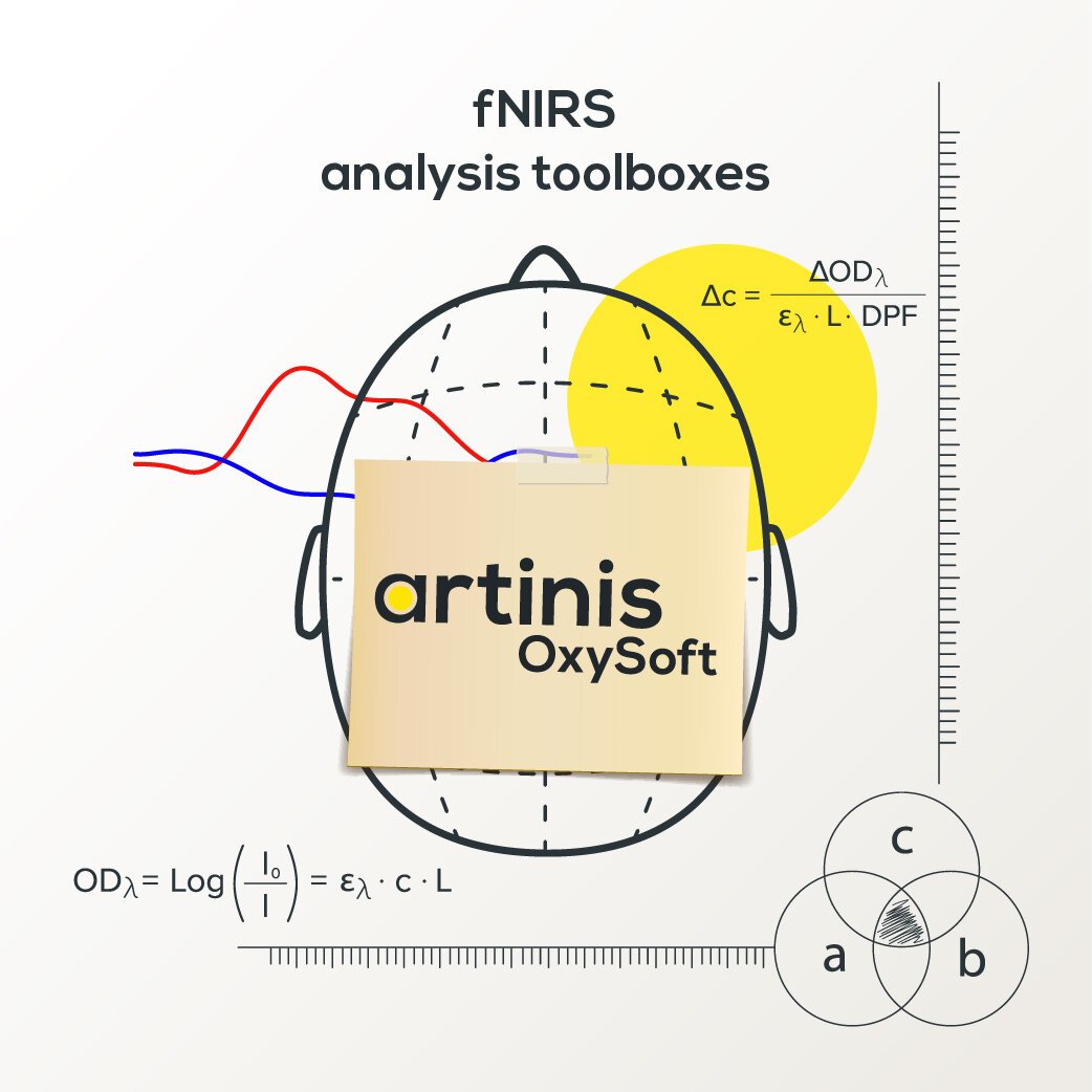
OxySoft
The software is used by all Artinis device users to collect, store, view, and analyze data. It is developed and maintained by the Artinis team.
Homer2 and Homer3
A MATLAB toolbox for analysis of fNIRS data and for creating maps of brain activation. The main developers of Homer are David Boas, Jay Dubb, and Ted Huppert, while several other people also contributed to writing specific function codes. Homer2 is the most used toolbox for fNIRS, which was recently updated to Homer3.
NIRSTORM
A NIRS analysis plugin for the MATLAB-based MEEG Brainstorm toolbox, the main developers are from different groups in Montreal, Paris, and Chemnitz.
NIRS-SPM
An SPM and Matlab plugin software package was developed for Statistical Parametric Mapping of NIRS by the BISP Lab and the Department of Bio and Brain Engineering in Korea.
FieldTrip
A MATLAB-based analysis toolbox that can be used for magnetoencephalography (MEG), electroencephalography (EEG), intracranial electroencephalography (iEEG), and fNIRS analysis. This toolbox was mainly developed in the Donders Institute for Brain, Cognition and Behaviour, the Netherlands, led by Robert Oostenveld and Jan-Mathijs Schoffelen.
BrainAnalyzIR
MATLAB-based analysis toolbox specifically tailored for fNIRS signal properties and statistical analysis, developed by Huppert Brain Imaging Lab.
MNE-NIRS
An extension of the MNE-Python toolbox for NIRS/fNIRSdata analysis, handled by scripting the processing pipeline in either a regular Python script or within a Jupyter notebook. This toolbox was developed by Robert Luke, Eric Larson and Alexandre Gramfort.
General workflow
Each toolbox works in their own distinct way, but the general workflow for all measurements is relatively similar. The order of the steps can be important and differs between the toolboxes. However, here we describe our suggested order of operations:
Acquiring the data
Hints and tips for data acquisition are outside the scope of this blog, but please do not hesitate to contact our application specialists for help.
Converting the data into a data format supported by a toolbox
Different toolboxes need the data to be represented in different data structures. Usually, the data structure comprises the raw optical data, the location of the channels, timestamps of the data and possible events. There are some standard formats, like .nirs which are used by multiple toolboxes. In 2019, the general file format .sfnirs for NIRS files was introduced. However, currently, different toolboxes use different file formats. At Artinis, we provide you with a dedicated Oxysoft2Matlab tool free of charge. This tool enables you to convert your Artinis data file to another file format.
Preprocessing of the data
Artefact handling
Parts of the data can be contaminated by artefacts, which could be systemic artefacts (e.g. heartbeat, respiration), or be caused by extrinsic factors (e.g. subject movement) (Tachtsidis&Scholkmann, 2016). Both these types of artefacts need to be handled separately. Usually, bad channels are removed first, which are channels with insufficient data quality (Sappia et al., 2020 and Sappia et al., 2021). Second, systemic and extrinsic artefacts need to be detected and handled. Artefact detection is often done by visual inspection of non-physiological data patterns or automated analysis using e.g. outlier detection using standard deviation. Artefact handling can be done in two ways: either, the data is removed from further analysis, or it is interpolated e.g. using cubic spline interpolation algorithm (Scholkmann et al., 2010).
Filtering
In a common analysis pipeline, fNIRS data is filtered such that the frequency of the hemodynamic response remains and frequencies of other signal components are filtered out. Although there are different opinions on the best filter cutoffs for estimating the hemodynamic response, most researchers filter out frequencies above 0.1 Hz (Pinti et al., 2018) in the healthy adult population. Other filter strategies can include a bandpass filter (Pinti et al., 2018), principal component analysis (Virtanen et al., 2009), or short channel regression (Zhang et al., 2007). In our blogpost series, we therefore mention what type of filter is used. Although the type of filter is of importance, most toolboxes do not leave a choice to the user. Details about the used filter are included in the specific toolbox blog posts.
Segmenting
The recorded data is segmented into those periods of experimental interest. The segmented period includes a few seconds before the task onset and a few seconds after the task offset.
Baselining and contrasting
The short period before the onset of the experimental task is usually used as a baseline. This allows making inferences between a baseline period (e.g. rest) and a task period (e.g. finger tapping). Alternatively, two task conditions can be contrasted directly without any other baseline period being necessary.
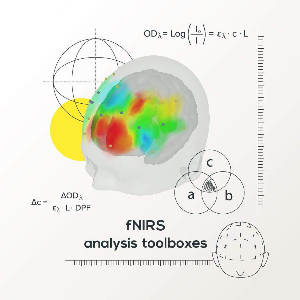
Conversion to concentrations
Traditionally, the modified Lambert-Beer law is used to convert from optical density as measured by the fNIRS device to relative changes in concentration of oxygenated and deoxygenated hemoglobin.
Averaging of data of interest
Averaging of data is usually first done across trials per condition, and, if available, over different sessions (also called runs), and then over subjects or per subject groups. In the data for our blog post series, we are analyzing data from a single subject performing the same task in multiple sessions.
Display
Displaying NIRS data is typically done by plotting both the average changes of oxy- and deoxyhemoglobin in time, often accompanied by error bars. These figures are widely used and accepted in scientific literature.
Additionally, many toolboxes offer the possibility to map the changes of oxy- and deoxyhemoglobin to specific regions of the brain. To do so one requires the relative position of the brain to the optodes and a brain template. More information about this can be found in our 3D-digitization blog post. Examples of toolboxes that can do this are OxySoft, Homer3 (through Atlasviewer), and NIRS-SPM.
There are two toolboxes (NIRStorm and Homer via AtlasViewer) that actually can compute the average lightpath of the photons and therewith estimate the source of the signal within an individual brain. This method requires individual MRI images, segmented and advanced Monte Carlo simulations (based on MCXlab) which are computationally expensive to compute, and are therefore implemenedt in specialized applications.
The dataset
Throughout all toolboxes, we will use a dataset that has been recorded with the Brite. This data set comprises 22 channels recorded over the motor cortex. We chose this dataset because it is a nice mix of typical NIRS-dataset properties. We see a clear and clean heartbeat in multiple channels. Furthermore, we have performed a typical finger-tapping experiment, which is well-known to cause a hemodynamic response in the motor cortex. Channel Rx7-Tx10 was positioned over the motor cortex so after analysis we evaluated the hemodynamic response in this channel. We performed the experiment across different sessions to illustrate how the toolboxes can be used to average over multiple datafiles. The processing pipeline will be kept as similar as possible for the different toolboxes to allow direct comparison between the different toolboxes.
Publish
Once the figures have been created, these can be used directly in a scientific article. Often the toolbox can provide additional statistical analysis as well. The goal of the upcoming blog posts is to provide the NIRS enthusiast with insight into which toolboxes he or she can use for which purpose. We hope these blogs provide a convenient overview and aid in improving data analysis methods for the whole NIRS field.
In this blog post, we present MNE-NIRS, a Python toolbox for analyzing NIRS/fNIRS data, which aims at researchers with a background in engineering, neuroscience and/or AI. The toolbox is handled by scripting the processing pipeline, which can be done in a regular Python script or within a Jupyter notebook.